User Guide
This guide provides an overview for working with the OptiDamTool package.
Verify Installation
To verify the installation, import the package and module and instantiate the classes using the following code. If no errors are raised, the installation is successful.
import OptiDamTool
watem_sedem = OptiDamTool.WatemSedem()
network = OptiDamTool.Network()
analysis = OptiDamTool.Analysis()
visual = OptiDamTool.Visual()
system_design = OptiDamTool.SystemDesign()
DEM to Stream
To generate the input files required to run the WaTEM/SEDEM model with the
river routing = 1 extension,
refer to the OptiDamTool.WatemSedem.dem_to_stream() method for more details on the output.
A sample Digital Elevation Model (DEM) raster file is available in the
data directory for testing purposes.
watem_sedem.dem_to_stream(
    dem_file=r"C:\users\username\input_data\dem.tif",
    flwacc_percent=1,
    folder_path=r"C:\users\username\output_folder"
)
Model Region Extension
To ensure compatibility with WaTEM/SEDEM, which does not support NoData cells, input rasters must be extended to include a buffer area beyond the original model region. This ensures that all computations are based on continuous data without missing values. A raster that covers the model region, typically the DEM raster, is used to create an extended region raster that includes the desired buffer zone.
watem_sedem.model_region_extension(
    dem_file=r"C:\users\username\input_folder\dem.tif",
    buffer_units=50,
    folder_path=r"C:\users\username\output_folder"
)
Using the region_buffer.tif raster generated by the OptiDamTool.WatemSedem.model_region_extension() method, other input rasters for WaTEM/SEDEM, such as the stream raster
produced in the DEM to Stream section, are spatially extended.
During this process, NoData areas are replaced with a specified fill value, resulting in a continuous raster suitable for further analysis.
watem_sedem.raster_extension(
    input_file=r"C:\users\username\output_folder\stream_lines.tif",
    fill_value=0,
    region_file=r"C:\users\username\output_folder\region_buffer.tif",
    output_file=r"C:\users\username\output_folder\stream_buffer.tif"
)
A constant raster, such as the erosion control factor,
is required for small regions when running WaTEM/SEDEM.
Using the region.tif and region_buffer.tif rasters generated by the OptiDamTool.WatemSedem.model_region_extension() method,
a constant-value raster can be created efficiently, as shown below:
watem_sedem.raster_constant_extension(
    input_file=r"C:\users\username\output_folder\region.tif",
    constant_value=1,
    region_file=r"C:\users\username\output_folder\region_buffer.tif",
    output_file=r"C:\users\username\output_folder\RUSEL_P_buffer.tif",
    fill_value=0,
    dtype='float32'
)
Raster Spatial Analysis
For focused spatial analysis, extracting a specific region from a large raster is often necessary. This function clips a raster using a rectangular bounding box derived from the total bounds of an input shapefile. If required, the shapefile’s Coordinate Reference System (CRS) is automatically transformed to match the CRS of the raster.
watem_sedem.raster_clipping_by_bounding_box(
    input_file=r"C:\users\username\input_folder\land_cover_ESRI.tif",
    shape_file=r"C:\users\username\output_folder\region_buffer.tif",
    output_file=r"C:\users\username\output_folder\land_cover_region.tif",
    dtype='int16'
)
After clipping, the output raster must be reprojected, clipped again, and rescaled in resolution to align with the model region. The input shapefile’s CRS and spatial extent are used for reprojection and spatial clipping. A mask raster, which shares the same extent as the shapefile, is used to rescale the resolution of the reprojected and clipped raster.
watem_sedem.raster_reproject_clipping_rescaling(
    input_file=r"C:\users\username\output_folder\land_cover_region.tif",
    resampling_method='nearest',
    shape_file=r"C:\users\username\output_folder\region.shp",
    mask_file=r"C:\users\username\output_folder\region.tif",
    output_file=r"C:\users\username\output_folder\land_cover_unprocessed.tif"
)
Land Cover Processing
To create land cover and management factor rasters required by WaTEM/SEDEM,
use the following codes and refer to methods OptiDamTool.WatemSedem.land_cover_esri()
and OptiDamTool.WatemSedem.land_management_factor() for more details.
# land cover raster
watem_sedem.land_cover_esri(
    lc_file=r"C:\users\username\output_folder\land_cover_unprocessed.tif",
    stream_file=r"C:\users\username\output_folder\stream_lines.shp",
    folder_path=r"C:\users\username\output_folder"
)

# land management factor
watem_sedem.land_cover_esri(
    lc_file=r"C:\users\username\output_folder\land_cover_unprocessed.tif",
    stream_file=r"C:\users\username\output_folder\stream_lines.shp",
    output_file=r"C:\users\username\output_folder\RUSLE_C.tif"
)
Product of Soil Erodibility and Rainfall Erosivity Factors
WaTEM/SEDEM uses the product of the Soil Erodibility (K) and Rainfall Erosivity (R) factors
when these values vary spatially across a large area. The multiplication is normalized by setting
the value of R to 1 where necessary. Refer to the method OptiDamTool.WatemSedem.rusle_kr() for more details.
watem_sedem.rusle_kr(
    k_file=r"C:\users\username\input_data\RUSLE_K.tif",
    r_file=r"C:\users\username\input_data\RUSLE_R.tif",
    region_file=r"C:\users\username\output_folder\region.tif",
    output_file=r"C:\users\username\output_folder\RUSLE_KR.tif",
    k_multiplier=1000
)
Raster Driver Conversion
WaTEM/SEDEM does not support raster files in the GTiff format. Therefore, input rasters must be converted to the Idrisi raster format with the .rst extension,
which is one of the two raster formats supported by WaTEM/SEDEM.
watem_sedem.raster_driver_to_rst(
    file_dict={'rusle_p': r"C:\users\username\output_folder\RUSEL_P_buffer.tif"},
    folder_path=r"C:\users\username\output_folder"
)
Adjacent Connectivity Between Dams
To determine the adjacent upstream and downstream connectivity between dams based on a stream network, a stream shapefile is required. This shapefile must contain a column representing a unique identifier for each stream segment.
Only one dam can be deployed per stream segment, and the dam is identified by the corresponding stream segment’s unique identifier. The specified stream segment identifiers are used to designate dam deployment locations.
A sample stream shapefile is available in the data directory. The examples below generate dictionaries representing the adjacent upstream and downstream connectivity of dams based on the stream network. A value of -1 indicates no downstream connectivity, while an empty list indicates no upstream connectivity.
# adjacent downstream connectivity
network.connectivity_adjacent_downstream_dam(
    stream_file=r"C:\users\username\input_folder\stream_lines.shp",
    dam_list=[21, 22, 5, 31, 17, 24, 27, 2, 13, 1]
)

# adjacent upstream connectivity
network.connectivity_adjacent_upstream_dam(
    stream_file=r"C:\users\username\input_folder\stream_lines.shp",
    dam_list=[21, 22, 5, 31, 17, 24, 27, 2, 13, 1]
)
Controlled Drainage Area of Dams
When working with a dam system within a stream network, the controlled upstream drainage areas for each dam are dynamically influenced by their specific locations. The following method calculate these areas.
network.controlled_drainage_area(
    stream_file=r"C:\users\username\input_folder\stream_lines.shp",
    dam_list=[21, 22, 5, 31, 17, 24, 27, 2, 13, 1]
)
Integration of Stream Information and Sediment Inflow Files
To support informed decision-making when deploying a dam system within a stream network, it is essential to have detailed information for each stream segment. This includes attributes such as stream connectivity, subbasin area, and sediment inflow. The following methods demonstrate how to generate a JSON file containing comprehensive stream segment data with sediment delivery values, and a GeoJSON shapefile that spatially represents sediment inflow for each segment. Sediment inflow into stream segments is computed using WaTEM/SEDEM with the extension Output per river segment = 1 enabled. For more details, refer to the method documentation.
# integrate sediment inflow to stream information TXT file
analysis.sediment_delivery_to_stream_json(
    info_file=r"C:\users\username\input_folder\stream_information.json",
    segsed_file=r"C:\users\username\input_folder\Total sediment segments.txt",
    cumsed_file=r"C:\users\username\input_folder\Cumulative sediment segments.txt",
    json_file=r"C:\users\username\output_folder\stream_with_sediment.json"
)

# stream shapefile with sediment inflow information
analysis.sediment_delivery_to_stream_geojson(
    stream_file=r"C:\users\username\input_folder\stream_lines.shp",
    sediment_file=rr"C:\users\username\output_folder\stream_with_sediment.json",
    geojson_file=r"C:\users\username\output_folder\stream_with_sediment.geojson"
)
Once the final stream GeoJSON file containing sediment inflow information is generated, it can be used to compute a summary of upstream metrics for selected dams. This includes identifying each dam’s directly connected upstream dams, calculating its controlled drainage area, and estimating the corresponding sediment inflow from that area. These metrics provide a comprehensive understanding of how the upstream network structure influences hydrological and sediment contributions to individual dam locations.
network.upstream_metrics_summary(
    stream_file=r"C:\users\username\output_folder\stream_with_sediment.geojson",
    dam_list=[21, 22, 5, 31, 17, 24, 27, 2, 13, 1]
)
To create a figure showing sediment inflow percentages to stream segments, relative to the total sediment input across all stream segments, use the following code:
visual.sediment_inflow_to_stream(
    stream_file=r"C:\users\username\output_folder\stream_with_sediment.geojson",
    figure_file=r"C:\users\username\output_folder\sediment_inflow_to_stream.png"
)
The following figure shows the output produced by the above code:

Dam System Storage Dynamics for Sedimentation
This method simulates the annual storage dynamics of a dam system affected by sedimentation. For each simulation year, the total sediment inflow to a dam is calculated based on two components: the sediment generated from the dam’s own drainage area and the sediment released from upstream dams.
The trapped sediment is determined by multiplying the total sediment inflow by the dam’s trap efficiency, which is a value between 0 and 1. At the end of each simulation year, the storage capacity of each dam is updated using a mass balance approach that accounts for the volume of sediment trapped.
When a dam becomes inactive, either because it has no remaining storage capacity or its sediment trapping efficiency falls below a defined threshold, the simulation dynamically updates the system. This includes adjusting system connectivity, recalculating controlled drainage areas, and updating sediment inflows to other dams in the network.
The simulation continues for a user-defined number of years or terminates early if either all dams become inactive or sediment release from the watershed exceeds the given threshold limit. The function returns a dictionary where each key corresponds to a DataFrame containing dam lifespan results, system-wide sedimentation statistics, individual dam performance metrics, and the simulation parameters used.
This method also provides an option to save the output dictionary to the input directory as a set of JSON files. Each file is named after a dictionary key and contains the corresponding DataFrame.
network.stodym_plus(
    stream_file=r"C:\users\username\output_folder\stream_with_sediment.geojson",
    storage_dict={
        21: 1500000,
        5: 100000,
        24: 60000,
        27: 200000,
        33: 1000000,
    },
    sediment_density=1300,
    trap_threshold=0.05,
    year_limit=100,
    write_output=True,
    folder_path=r"C:\users\username\output_folder"
)
To generate GeoJSON files of updated dam location points and their controlled drainage polygons when dams become inactive:
network.stodym_plus_with_drainage_scenarios(
    stream_file=r"C:\users\username\output_folder\stream_with_sediment.geojson",
    flwdir_file=r"C:\users\username\output_folder\flwdir.tif",
    storage_dict={
        21: 1500000,
        5: 100000,
        24: 60000,
        27: 100000,
        33: 1000000,
    },
    year_limit=15,
    sediment_density=1300,
    trap_threshold=0.05,
    folder_path=r"C:\users\username\output_folder"
)
Visualization of Dam System Simulation
This section presents visualizations of the simulated results generated in the Dam System Storage Dynamics for Sedimentation section.
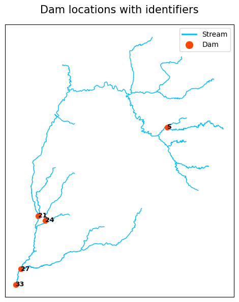
To create a figure showing dam locations along the stream path, use the following code:
visual.dam_location_in_stream(
    stream_file=r"C:\users\username\output_folder\stream_with_sediment.geojson",
    dam_file=r"C:\Users\username\output_folder\year_0_dam_location_point.geojson",
    figure_file=r"C:\users\username\output_folder\dam_location_in_stream.png"
)
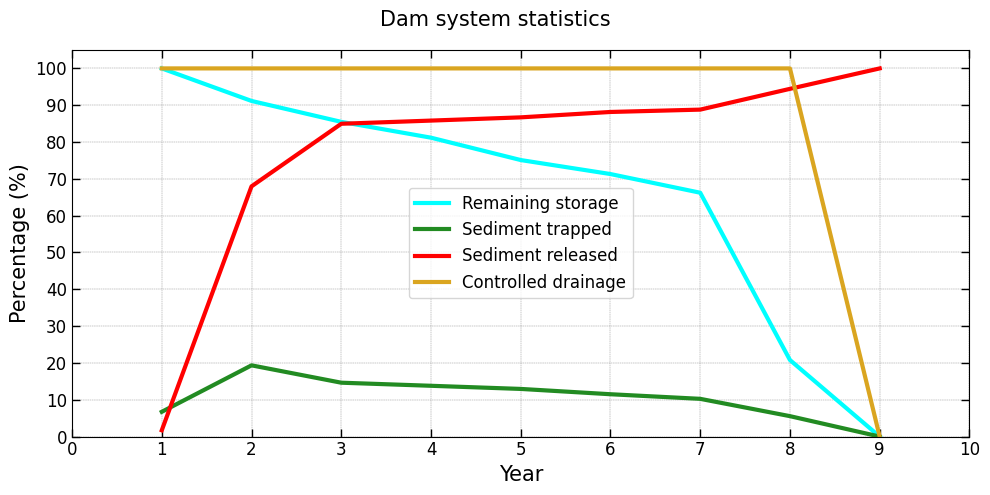
To generate a figure showing dam system-level statistics, including controlled drainage area, remaining storage, sediment trapped, and sediment released, use the following code:
visual.system_statistics(
    json_file=r"C:\users\username\output_folder\system_statistics.json",
    figure_file=r"C:\users\username\output_folder\system_statistics.png",
    ytop_offset=5,
    xtick_gap=1
)
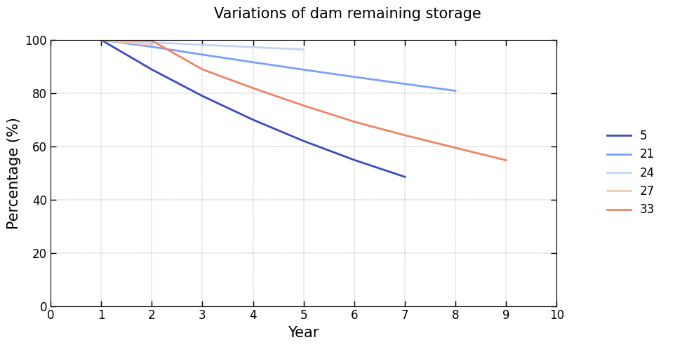
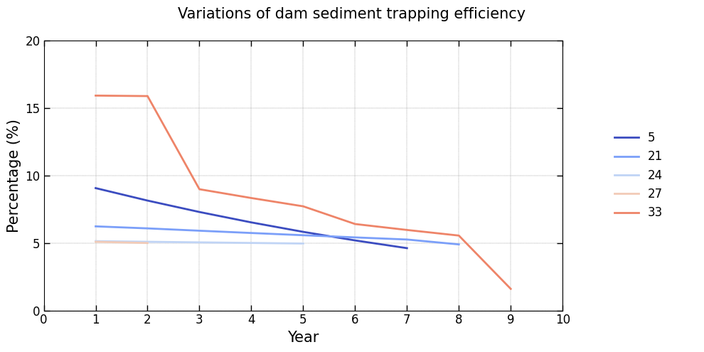
To generate figures illustrating the annual variability of key features for each dam in the system:
# dam remaining storage
visual.dam_individual_features(
json_file=r"C:\users\username\output_folder\dam_remaining_storage.json",
figure_file=r"C:\users\username\output_folder\dam_remaining_storage.png"
)
# dam sediment trapping efficiency
visual.dam_individual_features(
json_file=r"C:\users\username\output_folder\dam_trap_efficiency.json",
figure_file=r"C:\users\username\output_folder\dam_trap_efficiency.png"
)
# sediment trapped by dams
visual.dam_individual_features(
json_file=r"C:\users\username\output_folder\dam_trapped_sediment.json",
figure_file=r"C:\users\username\output_folder\dam_trapped_sediment.png"
)
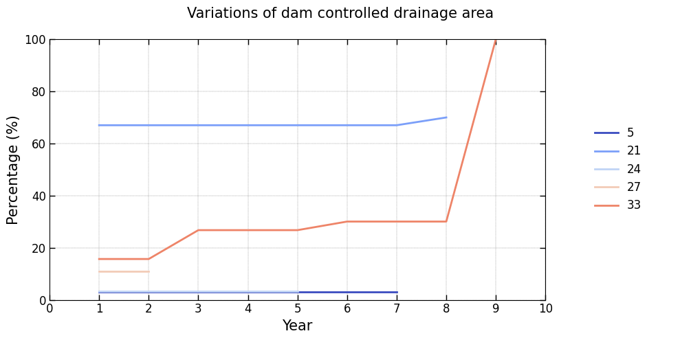
# dam controlled drainage area
visual.dam_individual_features(
json_file=r"C:\users\username\output_folder\dam_drainage_area.json",
figure_file=r"C:\users\username\output_folder\dam_drainage_area.png"
)

Optimizing Dam Systems for Sedimentation
Optimize dam locations and storage volumes within a watershed using a multi-objective evolutionary computation framework. The optimization is based on annual sediment inflow through watershed drainage pathways. Use the following code:
if __name__ == '__main__':
    output = system_design.sediment_control_by_fixed_dams(
        dam_number=5,
        storage_bounds=(1, 50),
        storage_multiplier=100000,
        stream_file=r"C:\users\username\output_folder\stream_with_sediment.geojson",
        stodym_config={
            'sediment_density': 1300,
            'year_limit': 100,
            'trap_threshold': 0.05,
            'brown_d': 1
        },
        objectives=[
            'drainage_area',
            'lifespan',
            'sediment_trapped_initial',
            'sediment_released_median',
            'curve_mean_deviation'
        ],
        algorithm_name='NSGAII',
        algorithm_config={
            'population_size': 10
        },
        nfe=100,
        seeds=4,
        folder_path=r"C:\Users\username\output_folder\dam_optimization",
        constraints={
            'lb_lifespan': 10,
            'ub_storage_sum': 10000000
        }
    )
Scenario Simulation from Optimized Solutions
To retrieve the detailed simulation outputs for a specific scenario obtained from the optimization process, use the following procedure. This allows you to reproduce the system behavior for any selected solution and inspect all associated performance metrics.
# storage dynamics
output = system_design.scenario_stodym_plus(
    solution_file=r"C:\Users\username\output_folder\dam_optimization\solutions_nondominated.json",
    count=0,
    stream_file=r"C:\users\username\output_folder\stream_with_sediment.geojson",
    stodym_config={
        'sediment_density': 1300,
        'year_limit': 100,
        'trap_threshold': 0.05,
        'brown_d': 1
    },
)

# storage dynamics and drainage response
output = system_design.scenario_stodym_plus_drainage_response(
    solution_file=r"C:\Users\username\output_folder\dam_optimization\solutions_nondominated.json",
    count=0,
    stream_file=r"C:\users\username\output_folder\stream_with_sediment.geojson",
    flwdir_file=r"C:\users\username\output_folder\flwdir.tif",
    folder_path=r"C:\Users\username\output_folder\dam_optimization\scenario_and_drainage",
    stodym_config={
        'sediment_density': 1300,
        'year_limit': 100,
        'trap_threshold': 0.05,
        'brown_d': 1
    }
)